ONERA OAT15A airfoil

Steady RANS of the ONERA OAT15A supercritical airfoil on structured grids, with DRAGonFLy’s \(p = 0\) solver. The case compares lift, drag and moment coefficients across grid levels at the transonic conditions of the OAT15A buffet test case, and the cost of each grid. The case lives in examples/ONERA-OAT15A/.

Note

The complete sweep so far is on ONERA’s Rizzi grids 1–7: all five angles of attack, 35 cases, all converged, at the DPW8 case 1a conditions. On the structured Cadence grids from the Eighth AIAA Drag Prediction Workshop (DPW8) only level 1 has been run, and only at \(\alpha = 1.36^\circ\) and \(1.50^\circ\). Comparisons with experimental data and other solvers will be added later.

Case

Geometry	ONERA OAT15A, chord 230 mm (scaled to 1 in the solver), blunt trailing edge
Mach number	\(M_\infty = 0.73\)
Reynolds number	\(Re = 3\times10^6\), based on the chord
Static free-stream temperature	271 K (Sutherland’s law), as in DPW8 test case 1a
Angles of attack	\(\alpha\) = 1.36°, 1.50°, 2.50°, 3.00°, 3.10°
Model	SA-neg RANS, cell-centred finite volume (\(p = 0\)), MUSCL inviscid fluxes
Boundary conditions	adiabatic no-slip wall; subsonic inflow/outflow far field (the inflow/outflow split, since replaced by the characteristic far field; these results predate the change)
Solver	pseudo-transient continuation (CFL\(_0\) = 5) to a residual of \(10^{-9}\), started from the converged first-order RANS solution
Moment reference	quarter chord, positive nose-up

Cases run one at a time. Each starts from the converged first-order solution of the same model: the RANS solve without MUSCL, itself started from the free stream, on the same mesh and angle of attack (--init first-order, the default). In the one case tested, REV02 Level 1 at \(\alpha = 1.36^\circ\), this took 98 MUSCL pseudo-time steps against 180 from the free stream, and the converged solution is the same to the printed digits. The Rizzi results below were computed before this option existed and start from the free stream.

Obtaining the meshes

The meshes are not stored in the repository. The case uses the structured Cadence grids from DPW8:

1. Download Cadence-ONERA-OAT15A_230mmChord_780mmSpan_upZ_2024_09_05_Structured.zip (554 MB) from https://dpw.larc.nasa.gov/DPW8/ONERA_OAT15A/Cadence_Grids.REV01/. This directory can also be reached from the DPW8 grid page, https://www.aiaa-dpw.org/grids.html. The same directory has an _Unstructured.zip; the case does not use it.

2. Unzip it in the repository’s meshes/ directory:

   $ cd meshes
   $ unzip Cadence-ONERA-OAT15A_230mmChord_780mmSpan_upZ_2024_09_05_Structured.zip
   

   This creates meshes/Cadence-ONERA-OAT15A_230mmChord_780mmSpan_upZ_2024_09_05_Structured/. The case reads only the .cgns files in it, ONERA-OAT15A_230mmChord_780mmSpan_upZ_2024_09_05_Structured_Level-N.cgns for N = 1 to 6. The .ugrid, .mapbc and .pw files, and the __MACOSX folder the archive may contain, are not needed.

To keep the meshes elsewhere, pass that directory with --mesh-dir.

The Rizzi grids (--mesh-family rizzi), used for the complete sweep below, are in https://dpw.larc.nasa.gov/DPW8/ONERA_OAT15A/ONERA-Rizzi_Grids.REV00/. The case expects them at meshes/ONERA-ONERA-OAT15A-Rizzi/gridN/OAT15A_Rizzi_N.cgns, for N = 1 to 7 (see also meshes/README.md).

Grids

Each Cadence grid is a structured multi-block CGNS grid: 6 blocks, 3D, and one cell thick in span. dragonfly_sim.utils.mesh_io_utils reads it with PyVista and reduces it in memory to the 2D quadrilateral mesh the solver uses: it keeps one span plane of every block and merges the nodes the blocks share. No converted mesh file is written. At \(p = 0\) with SA-neg, each cell carries 5 unknowns.

Level	Cells	Degrees of freedom	Wall edges
1	151,003	755,015	703
2	240,554	1,202,770	842
3	378,312	1,891,560	976
4	596,792	2,983,960	1,110
5	937,027	4,685,135	1,239
6	1,471,296	7,356,480	1,371

The first cell at the wall is about \(7\times10^{-6}\) chords high on level 1 and \(2\times10^{-6}\) chords on level 6. The far field is about 150 chords from the airfoil.

The Rizzi grids have the same layout (4 blocks, one cell thick in span) and are read the same way. Their first cell is about \(10^{-5}\) chords high on every level, and their far field is about \(5\times10^4\) chords away.

Grid	Cells	DOFs
1	15,872	79,360
2	34,816	174,080
3	63,488	317,440
4	100,352	501,760
5	144,384	721,920
6	253,952	1,269,760
7	471,040	2,355,200

Results

Rizzi grids 1–7

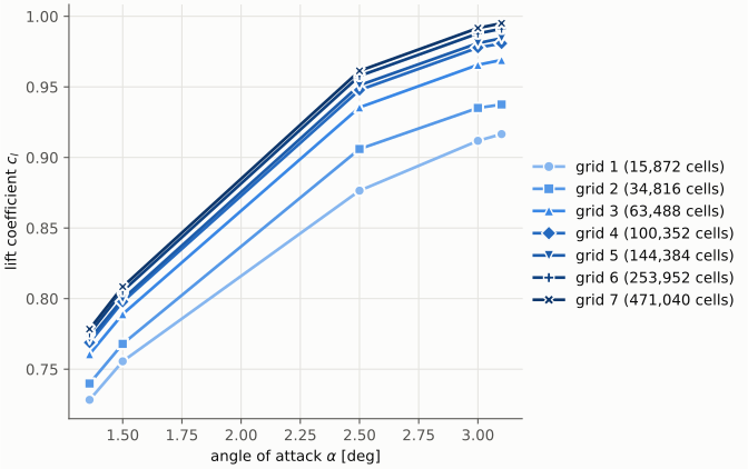
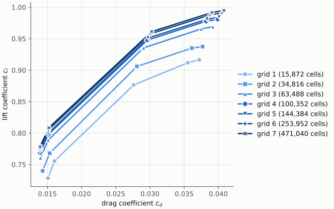
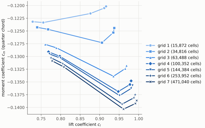
All 35 cases (7 grids at 5 angles of attack) converged to a residual below \(10^{-9}\), at 271 K. They were run on a computing cluster (TSCC) with 8 MPI ranks, one case at a time, each from the free stream. Each line in the first three figures is one grid’s angle-of-attack sweep, from the coarsest grid (light) to the finest (dark). Hollow markers would mark cases that did not converge.

Lift coefficient against angle of attack

Lift coefficient against drag coefficient

Moment coefficient against lift coefficient

Finest grid and grid convergence

Grid 7 (471,040 cells), with its drag split into the pressure and friction parts, and how much the coefficients still change from grid 6 to grid 7:

\(\alpha\)	\(c_l\)	\(c_d\)	pressure	friction	\(c_m\)	\(c_l\) change, grid 6 → 7	\(c_d\) change, grid 6 → 7
1.36°	0.7784	0.01393	0.00726	0.00666	−0.1309	+0.0030 (+0.38%)	+0.1 counts
1.50°	0.8085	0.01520	0.00861	0.00659	−0.1321	+0.0031 (+0.38%)	+0.3 counts
2.50°	0.9614	0.03025	0.02420	0.00605	−0.1403	+0.0036 (+0.37%)	+2.0 counts
3.00°	0.9917	0.03907	0.03328	0.00579	−0.1392	+0.0038 (+0.39%)	+2.7 counts
3.10°	0.9951	0.04082	0.03508	0.00574	−0.1387	+0.0039 (+0.39%)	+2.9 counts

• Lift keeps rising with refinement: from grid 1 to grid 7 it increases by 0.05 at 1.36° and by 0.08 at 3.1°. From grid 6 to grid 7 the change is still about 0.4% at every angle, so the sweep is not grid converged in \(c_l\) at the 0.5% level.

• Drag is converged to within 3 drag counts (\(3\times10^{-4}\)) between the two finest grids, with the largest change at the highest angles of attack. The friction part varies very little across all grids (0.00666 to 0.00659 at 1.50°); the pressure part carries the changes.

• Moment: the pitching moment becomes more nose-down with refinement and changes by about 0.001 from grid 6 to grid 7.

• The complete results (every grid and angle) are in examples/ONERA-OAT15A/data/rizzi_results.csv.

Cost: wall time against degrees of freedom

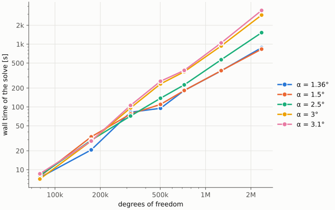
Wall time of the steady solve (pseudo-transient continuation only, without model set-up and output), one line per angle of attack. Both axes are logarithmic.

Pseudo-time steps and solve wall time per case:

Grid	DOFs	1.36°	1.50°	2.50°	3.00°	3.10°
1	79,360	37 / 8 s	37 / 8 s	44 / 8 s	38 / 7 s	45 / 9 s
2	174,080	50 / 21 s	101 / 33 s	89 / 30 s	88 / 29 s	83 / 29 s
3	317,440	114 / 82 s	105 / 77 s	114 / 72 s	140 / 96 s	141 / 106 s
4	501,760	68 / 95 s	82 / 110 s	126 / 138 s	196 / 232 s	208 / 257 s
5	721,920	113 / 183 s	108 / 183 s	116 / 225 s	179 / 364 s	199 / 382 s
6	1,269,760	134 / 376 s	137 / 379 s	179 / 566 s	291 / 937 s	315 / 1046 s
7	2,355,200	166 / 879 s	150 / 833 s	232 / 1526 s	458 / 2909 s	575 / 3448 s

• The sweep took 4.4 hours of wall time in total.

• The cost depends strongly on the angle of attack. The lower angles take 150–230 steps on the finest grid; at 3.0° and 3.1°, approaching the angles where this airfoil buffets (the DPW8 case extends to 3.9°), the step count grows with refinement, to 458 and 575 steps on grid 7. A step costs about 5–6 s on grid 7.

• Wall time grows roughly as DOFs\(^{1.2}\) at 1.36° and DOFs\(^{1.7}\) at 3.1° (grids 3 to 7).

Cadence grids

Level 1, 8 MPI ranks of an Intel Core i7-10700 (8 cores), 8.8 GiB of memory in total. These two cases were run at 300 K; at 271 K the coefficients change by about \(10^{-4}\) (tested on Rizzi grid 1):

\(\alpha\)	PTC steps	Solve wall time	\(c_l\)	\(c_d\) (friction)	\(c_m\)
1.36°	415	1981 s	0.7605	0.01363 (0.00648)	−0.1280
1.50°	560	2996 s	0.7901	0.01478 (0.00642)	−0.1288

On this grid the residual stalls for long stretches (around \(10^{-3}\), then \(10^{-5}\)) before it converges, so each case takes several hundred pseudo-time steps.

Comparison with experiment and other solvers

To be added.

Running

The full sweep, Cadence levels 1–6 at all five angles of attack, one case at a time:

$ cd examples/ONERA-OAT15A
$ OMP_NUM_THREADS=1 mpirun -n 8 python oat15a_analysis.py --out-dir <output folder>

Each run writes a new folder under --out-dir containing:

• results.csv: one row per case, rewritten after every case. Columns: grid, cells, dofs, alpha, converged, steps, residual, wall_s (the solve), case_s (model set-up + solve), \(c_l\), \(c_d\) and its pressure and friction parts (c_d_pressure + c_d_friction = c_d), \(c_m\).

• wall_gridN_aA.csv: wall \(C_p\) and \(c_f\) at the ends and middle of every wall facet.

• solution_gridN_aA.npz: the converged solution of each case, with its settings. It is written with dragonfly_sim.utils.checkpoint.save_checkpoint and does not depend on the number of MPI ranks. To post-process a case (for example \(C_p\) in the field), rebuild the model on the same grid and fill it with load_checkpoint.

• The four figures of the Rizzi results above, in that same folder. With --write-fields, also VTX files of the solution, pressure and Mach number for ParaView.

Useful options:

• --grids and --alphas run a subset, for example --grids 1 2 --alphas 2.5.

• --mesh-family rizzi runs the Rizzi grids 1–7 instead.

• --init {first-order,rans1,euler,freestream} selects the starting state: the first-order RANS solution (the default for the RANS model), the first-order RANS or Euler solution by name, or the free stream (the default for --model euler). --init-tol and --init-max-steps control the first-order solve; its wall time is reported in results.csv as init_s and init_steps.

• --model euler runs the Euler equations (slip wall, no turbulence model) instead of SA-neg RANS: the first-order model (HLL flux) by default, started from the free stream. --muscl adds MUSCL reconstruction, with the Van Albada limiter, \(\epsilon = 0.1\), as its default slope limiter (--limiter, --limiter-eps; the RANS model defaults to no limiter). The MUSCL Euler model is fragile on the Rizzi grid 1 at \(\alpha = 2.5^\circ\), and the results should be treated as experimental. Without a limiter it ended in a positivity-limiter freeze. With the Van Albada limiter it reached one of two different converged steady states, with the upper-surface shock at \(x = 0.714\) (\(c_l = 1.2245\)) or at \(x = 0.684\) (\(c_l = 1.1977\)), both to a residual below \(10^{-9}\); in one run it did not converge in 921 steps. The number of steps varies as well (166 to 610 for converged runs), and runs with identical settings did not always give the same outcome. The RANS model, in contrast, gave identical coefficients from every starting state tested. --init euler starts the MUSCL Euler model from the first-order Euler solution.

• --cfl-rise-min and --cfl-rise-max set how much the pseudo-time CFL number is cut when the residual rises (default: by the residual ratio, between 0.7 and 0.9).

• --mesh-dir points at meshes kept outside meshes/.

The SA-neg model, the mesh input and the force coefficients come from examples/flow_analysis.py and the dragonfly_sim package.

Warning

The finer Cadence levels are expensive. On level 1, each case took 33–50 minutes on 8 ranks and 8.8 GiB of memory. Memory grows roughly with the number of degrees of freedom, so level 6 (about 10 times level 1) is expected to need more memory than a 46 GB workstation has. This is an estimate, not a measurement.

To redraw the figures from a results file:

$ python oat15a_analysis.py --plot <run folder>/results.csv --figure-dir figures

Figures are SVG by default. Use --format pdf (or png) for other uses.