Examples

Both examples live in examples/ of the repository and run on the bundled NACA 0012 (chord 1 m, flow along +x, 4,032-cell one-cell-thick mesh with 126 faces on the airfoil). They are written for mpirun -np 4; the case is re-decomposed for whatever rank count you launch with. Every number and figure below comes from a real run (DAFoam 5.1.1, ARM64 Linux, 4 ranks); Verification status says what each rests on.

Analysis: airfoil_analysis.py

mpirun -np 4 python examples/airfoil_analysis.py                      # Euler mode, alpha = 3 deg
mpirun -np 4 python examples/airfoil_analysis.py --case naca0012      # RANS, wall function
mpirun -np 4 python examples/airfoil_analysis.py --aoa 1.5
mpirun -np 4 python examples/airfoil_analysis.py --check-totals       # adjoint vs finite differences

Expected output (Euler mode, 3 degrees, 238 m/s; it takes seconds):

case=naca0012_euler  warper=jax  alpha=3.0 deg
  CL = 0.47056
  CD = 0.011743  (117.4 counts)
saved analysis.png (C_p contours and surface C_p)

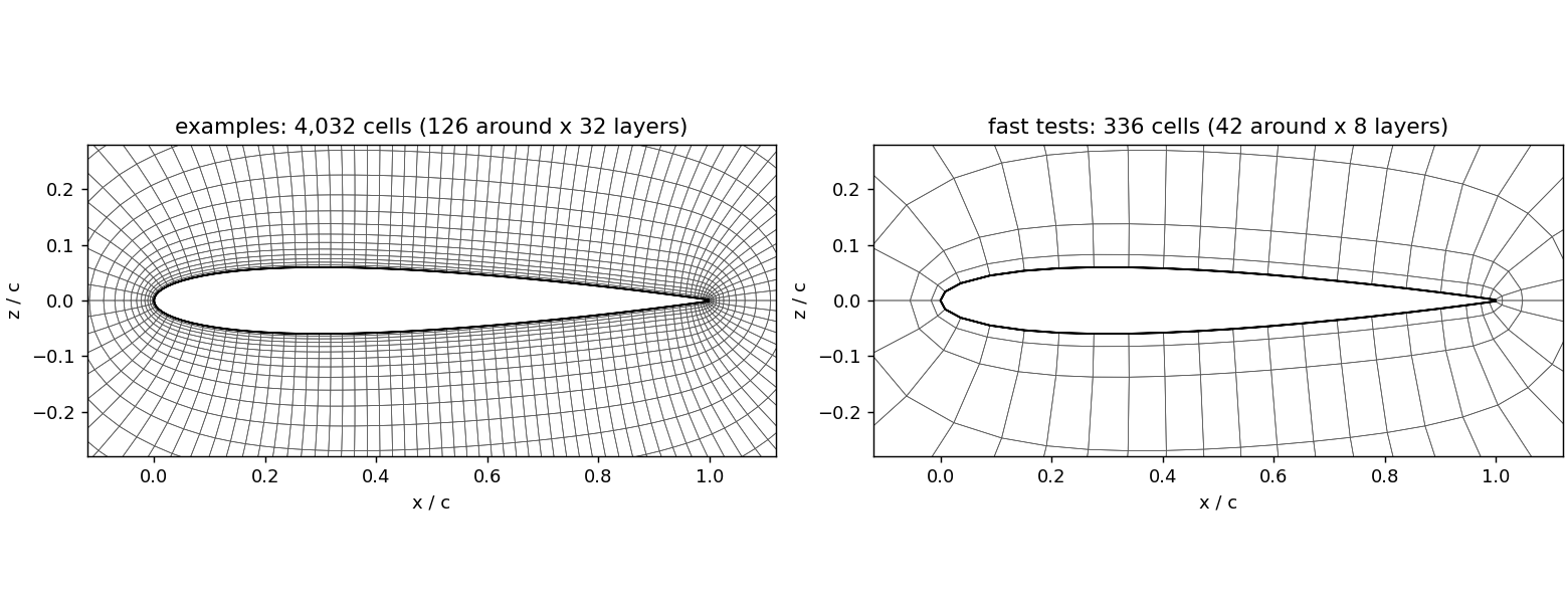
The bundled mesh (left) and the 336-cell mesh the fast tests use (right).

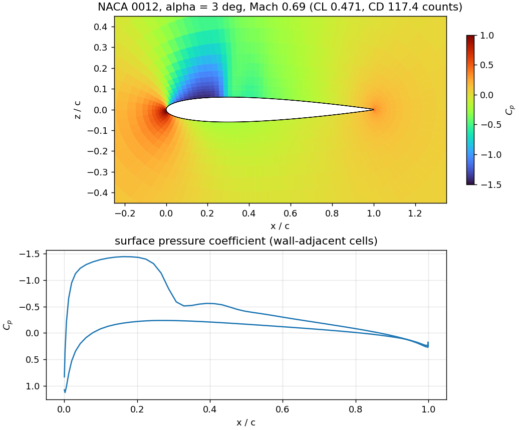
The upper surface has a suction peak (C_p = -1.45) ending in a sharp jump at 30% chord: a shock, on a NACA 0012 at 3 degrees and Mach 0.69. That is where the drag comes from, and what the optimization removes.

--check-totals additionally compares the adjoint derivatives of CD and CL with respect to the six shape variables and the angle of attack with finite differences (step 0.01), one flow solve per variable per step: the quickest way to confirm that a new case or option set produces trustworthy gradients before you spend an optimization on it. On the bundled case the two agree to 0.2 to 2% (below a step of about 1e-3 the finite differences are noise; see Verification status).

Walk-through. The script is a thin shell around the library: prepare_case copies and decomposes the case, build_airfoil_model builds the CSDL model (geometry, mesh warp, DAFoam solve), model.analyze() runs it and returns CL and CD, and viz draws the result. The same few lines are in Quickstart.

Optimization: airfoil_optimization.py

mpirun -np 4 python examples/airfoil_optimization.py --maxiter 100    # Euler mode (default case), 100 iterations: 37 min; same design by iteration 65 (13 min)
mpirun -np 4 python examples/airfoil_optimization.py --maxiter 40     # about 7 min; still improving
mpirun -np 4 python examples/airfoil_optimization.py --case naca0012  # the original RANS tutorial setup
mpirun -np 4 python examples/airfoil_optimization.py --no-movie       # skip the movie (the figures are still written)

Minimizes CD subject to CL = 0.5 (--cl-target) with DAFoam adjoint gradients. The stack is exactly the lab’s: lsdo_geo parameterizes the geometry, IDWarp-JAX deforms the volume mesh, DAFoam solves the flow and adjoint, CSDL assembles the derivatives, and modOpt’s OpenSQP optimizes.

mpirun -np 4 python examples/airfoil_optimization.py --optimizer PySLSQP   # SLSQP instead of OpenSQP
mpirun -np 4 python examples/airfoil_optimization.py --warper idwarp       # Fortran IDWarp instead of IDWarp-JAX
mpirun -np 4 python examples/airfoil_optimization.py --adjoint-tol 1e-3    # 29% faster adjoints (measured on one gradient; not run through a full optimization)

Result of the 100-iteration run (Euler-mode case, IDWarp-JAX, OpenSQP, 4 ranks):

  initial: CL = 0.47056  CD = 117.4 counts
  final:   CL = 0.50000  CD = 75.4 counts
  CD change: -35.8 %
  thickness: [19.6464 35.6686 33.9458]     (percent change at the three interior control points)
  camber: [ 4.1915  8.1936 11.2012]
  angle_of_attack: [0.]                     (at its lower bound)

The movie shows every optimizer iteration: pressure-coefficient contours, surface C_p and the airfoil shape (the initial ones in grey), then the histories of CD, CL, optimality and feasibility with a marker at the current iteration.

The design that results is visibly thicker, more cambered, and flown at zero angle of attack: the strong suction peak and shock are replaced by a gently loaded, shock-free upper surface that carries the same lift.

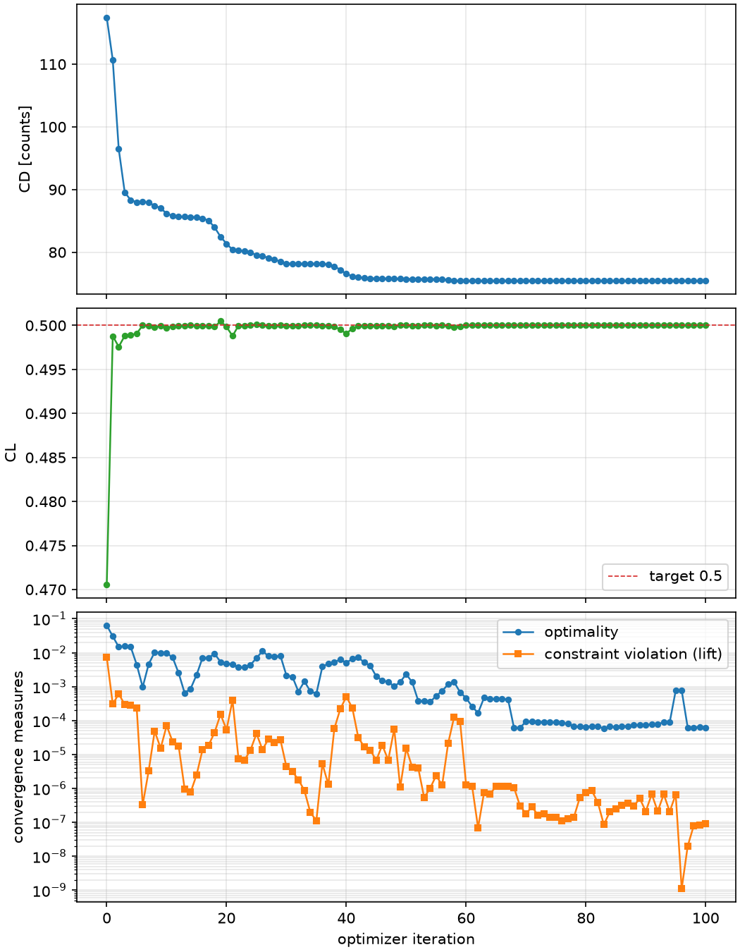
CL reaches its target within six iterations and stays there. Drag falls in steps and stops changing at about iteration 65 (75.42 counts). Optimality reaches about 6e-5 but not the default 1e-5, so modOpt reports “not converged” at the iteration cap even though the objective no longer moves; the brief optimality spike near iteration 95 is a transient that the optimizer recovers from within two iterations.

Cost, and when to stop

The 100-iteration run took 36.7 minutes of optimizer time (4 ranks, 4,032 cells). Most of it bought nothing:

Iteration	Elapsed	CD (counts)	Function evaluations	Gradient evaluations
10	2.1 min	86.2	17	15
20	3.5 min	81.4	27	25
40	7.0 min	76.55	52	50
65	13.0 min	75.42	106	92
80	24.7 min	75.42	233	167
100	36.7 min	75.42	406	244

CD stops changing at iteration 65 (13 minutes); the remaining 24 minutes polish an unchanged design. Early iterations cost about 10 s each and the last ones about 40 s, because the line search takes many steps once the optimizer is creeping along a flat valley (iterations 80 to 100 needed 173 function and 77 gradient evaluations). For this case --maxiter 65 gives the same design in about a third of the time. A looser --tolerance might stop it earlier, but optimality plateaus near 6e-5, so the default 1e-5 is never met and a value such as 1e-4 would need to be tried before relying on it.

Reading it carefully: the mesh is coarse (4,032 cells) and the Euler-mode case has no resolved boundary layer, so the absolute drag numbers are not physical and the optimum partly exploits the mesh (Verification status). It is a demonstration of the workflow, not a design.

OpenSQP is modOpt’s own SQP implementation (BFGS Lagrangian-Hessian approximation, an elastic-mode merit function that tolerates infeasible QP subproblems, and HiGHS for the QPs). --maxiter counts major iterations and --tolerance sets both its optimality and feasibility tolerances (acc for PySLSQP). Further OpenSQP options (verbosity, ls_maxiter, …) pass through AirfoilModel.optimize(**solver_options).

Design variables (7):

Variable	Count	Meaning	Bounds
thickness	3	percent change of the local FFD block thickness at the three interior chordwise control points	-100 to 100
camber	3	vertical shift of the same control points, in percent of the control-point spacing (chord/4 for the default 5 points; see How it works)	-50 to 50
angle_of_attack	1	degrees	0 to 10

Outputs, in the working directory (run/ by default): optimized_airfoil.npz (initial and optimized surface coordinates and the design variables), history.npz and history.png (CD, CL, and the solution kept for each iteration), optimization.png, movie.gif and, if ffmpeg is installed, movie.mp4, and ASO_2DAF_rank0_outputs/ (modOpt’s own iteration history).

Walk-through. model.optimize(sim, algorithm="OpenSQP", maxiter=...) wraps the simulator in a modOpt problem; it records CD and CL at every gradient evaluation (model.history), and viz.make_movie draws the frames from the solutions DAFoam keeps on disk (about 0.2 s per frame), so the movie costs the optimization nothing.

What “Euler mode” means here

DAFoam’s compressible solver DARhoSimpleCFoam always carries viscous terms and a turbulence model. To approximate inviscid (Euler) flow, the naca0012_euler case takes the RANS case and:

• lowers the constant dynamic viscosity from 1.8e-5 to 1.8e-9 kg/(m s), so the chord Reynolds number rises from about 1.5e7 to about 1.5e11, and scales the Spalart-Allmaras seed (nuTilda, nut) down by the same factor 1e4;

• keeps the bundled coarse mesh. At this Reynolds number the boundary layer is far thinner than the first cell, so with the wall function it carries almost no shear: lift is essentially pressure lift and drag is wave drag plus the numerical dissipation of the scheme.

The point is a cheap case (no resolved boundary layer, quick primal and adjoint) in which shock-related drag dominates, so shape changes that weaken the shock show up clearly in CD. Two caveats follow from it. CD from this case is not a physical drag (there is no skin friction, and the numerical dissipation depends on the mesh), so compare designs within the case rather than against experiment. And a coarse mesh is a compromise: optimizers exploit mesh-resolution artifacts, so check any promising shape on a finer mesh or in RANS.

Your own case

Copy the examples and replace the three ingredients:

1. an OpenFOAM case directory for DARhoSimpleCFoam (or adapt options.naca0012_options),

2. a STEP file of the same geometry (lsdo_geo projects the CFD surface onto it),

3. a DAFoam options dictionary whose inputInfo uses only the input types the interface builds (volCoord, patchVelocity, patchVar for p and T).

For a different parameterization, call the pieces in How it works directly instead of build_airfoil_model.

Timings (measured)

On an Apple M5 Max (12 cores), in the Linux VM of Installing on an Apple-silicon Mac, one analysis or optimization iteration costs:

	4,032-cell mesh, 1 rank	4,032-cell mesh, 4 ranks	336-cell test mesh
build the model (geometry, projection, IDWarp-JAX, DAFoam start-up, first solve)	9 s	5 s	3 s
forward solve after an optimizer-sized design change (warm-started)	3.9 s	1.4 s	0.2 s
adjoint derivatives (CD and CL) at the base design		7 s	0.7 s
… at a design with a stronger shock (CL 0.58)	101 s	31 s
first compute_totals (adds a one-time ~5 s JAX compile)		about 17 s (not re-timed since a bug fix; see Verification status)	5.6 s

The adjoint dominates and depends on the flow state: it takes 260 GMRES iterations per output at an easy state and many more near a shock. Four ranks give about 3.3x over one on the 4,032-cell mesh; the 336-cell mesh is too small to gain from more ranks. The complete optimizations on the 4,032-cell mesh, 4 ranks: 40 iterations, 50 gradient evaluations, 430 s (7 min); 100 iterations, 36.7 minutes (the movie above; later iterations cost more because the adjoint is harder near the final shape); about a second per iteration on the 336-cell mesh. Nothing here uses a GPU: DAFoam and OpenFOAM are CPU-only.

Speeding it up

Measured on the 4,032-cell mesh, 4 ranks, at one design, adjoint only (scripts/vm/timing.py with environment settings):

Change	Adjoint time	Derivatives vs the default (max relative difference)	Verdict
default (adjoint tolerance 1e-6)	7.0 s
adjoint tolerance 1e-4	5.6 s (-20%)	3e-5	free
adjoint tolerance 1e-3	5.0 s (-29%)	7e-4	good; use --adjoint-tol 1e-3
preconditioner recomputed every 3rd evaluation (adjPCLag)	8.8 s (+26%)	4e-7	slower here; do not
primal tolerance 1e-6 (default 1e-8)	forward solve 1.0 s instead of 1.4 s	7e-3	not worth the gradient error

Finite-difference noise on these derivatives is about 1e-2, so the looser adjoint tolerances change nothing that matters to the optimizer. Other levers, not measured here: the 336-cell mesh for exploring (about 10x cheaper per iteration, but crude); fewer or better-scaled design variables; and, for large 3D meshes, more ranks. A looser optimizer tolerance will not shorten the 40-iteration optimization by itself: it never met the default tolerance, and it plateaued for five iterations (31 to 35) before improving again, so a looser tolerance risks stopping at the plateau.