Steps for solving a topology optimization problem in ATOMiCS¶

The users just need to modify the run_files (see Examples library) to perform a topology optimization. We present an introduction to the settings of the run_files below.

1. Define the mesh¶

ATOMiCS supports FEniCS built-in meshes as well as external mesh of .vtk or .stl type from GMSH, pygmsh or other mesh generation tools.

1.1 FEniCS built-in meshes:

The documentations for FEniCS built-in meshes can be found here.

1.2. External mesh:
We use meshio to convert the external mesh to the formats that FEniCS accepts (.vtk or .stl for now). GMSH can be installed from here.

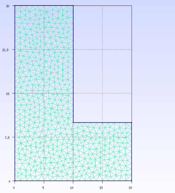
An example mesh generated from GMSH GUI is shown below:

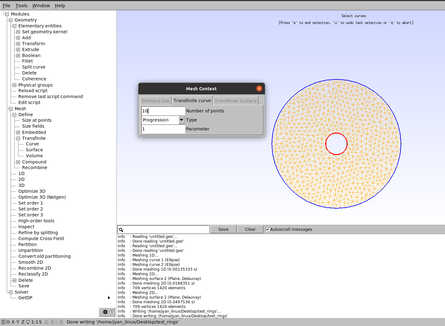
Here is one of the GMSH tutorials you can find online. One important thing to note is that you need to try to generate meshes that are close to the same size to make the filter to work properly. This can be done in a couple of ways in GMSH. One way to do it is Mesh->Transfinite->line/curve and tune the number of points on different sides.

After generating the mesh, we need to export the mesh into .vtk or .stl format (ctrl+e for GMSH) in the same folder as your run_file. Then, we use meshio to convert the file to .vtk or .stl format using the code below (see Topology optimization using external mesh)
# import the mesh file generated from your external tool
import meshio
filename = <file_name>
mesh = meshio.read(
    filename,
    file_format=<file_format> # "vtk" or "stl" are tested
)

# convert the mesh into xml
meshio.write_points_cells(
    <out_file_name>, # "fenics_mesh_l_bracket.xml"
    mesh.points,
    mesh.cells,
    )

# set the mesh as input to the topology optimization problem
mesh = df.Mesh(<out_file_name>)
GMSH and pygmsh may automatically generate 3D mesh even if you set it to 2D. You can varify this by using d=len(displacements_function). if d=3, you may want to convert this to 2D using the code below instead (see Case study II: battery pack topology optimizations). (Importing os may cause some error for openmado n2 file_name.py for visualizing the code structure. If that happens, you can generate the mesh in a seperate python file. Then, just use the last line of code in the run file.)
filename = 'name.vtk'
mesh = meshio.read(
    filename,
    file_format="vtk"
)

import os
os.system('gmsh -2 name.vtk -format msh2')
os.system('dolfin-convert name.msh name.xml')
mesh = df.Mesh("name.xml")

2. Setting the boundary conditions¶

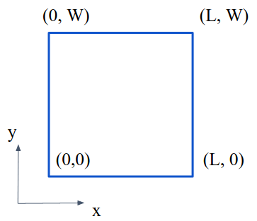
We use FEniCS built-in functions to define boundary conditions for the topology optimization problems. Below is a quick demonstration using a simple 2D square.

class LeftBoundary(df.SubDomain):
    def inside(self, x, on_boundary):
        return (abs(x[0] - 0)< df.DOLFIN_EPS)

class RightBoundary(df.SubDomain):
    def inside(self, x, on_boundary):
        return (abs(x[0] - L)< df.DOLFIN_EPS)

class BottomBoundary(df.SubDomain):
    def inside(self, x, on_boundary):
        return (abs(x[1] - 0)< df.DOLFIN_EPS)

class TopBoundary(df.SubDomain):
    def inside(self, x, on_boundary):
        return (abs(x[1] - W)< df.DOLFIN_EPS)

The functions above captures the left, right, bottom, and top boundary, respectively. FEniCS uses x[0], x[1], `` x[2]`` to represent x, y, and z.

Then, the users can add the boundary conditions to the problem using the code below:

bc_left = df.DirichletBC(function_space, df.Constant((0.0)), LeftBoundary())
bc_bottom = df.DirichletBC(function_space.sub(0), df.Constant((0.0)), BottomBoundary())

pde_problem.add_bc(bc_left)
pde_problem.add_bc(bc_bottom)

Note that the function_space.sub(0) here represents the x component of the function space. If the function_space is for a displacements field, the bc_bottom is a sliding boundary condition to constrain the x displacements meaning the structure can only slide in y direction on the bottom boundary of the square. While the bc_left is a clamped boundary meaning all the displacements on the left boundary are set to zeros.

3. Select a filter¶

The users can choose between a linear direct filter implemented in OpenMDAO and a FEniCS variational filter. For now, we recommand the linear direct filter.

from atomics.general_filter_comp import GeneralFilterComp
from atomics.pdes.variational_filter import get_residual_form_variational_filter

4. Select a penalization scheme¶

The users can choose between SIMP and RAMP method by specifying the <method_name>.

residual_form = get_residual_form(
    ...,
    method=<method_name>
    # <method_name> can be 'SIMP' or 'RAMP'
)

5. Solve for the states¶

First, on the top of the run_file, the users need to import the corresponding PDE.

from atomics.pdes.<pde_name> import get_residual_form

Then, we need to specify the inputs for get_residual_form. The users can do a ctrl+click to see what variables should be specified.

residual_form = get_residual_form(
    ...,
)

6. Select solvers for the FEA problem and the adjoint equation¶

This setting can be modified by changing the options in AtomicsGroup in the run_file.

group = AtomicsGroup(pde_problem=pde_problem,
                     linear_solver=<solver_name>,
                     problem_type=<prob_type>,
                     ...)

There are currently six options (fenics_direct, scipy_splu, fenics_krylov, fenics_krylov, petsc_gmres_ilu, scipy_cg, petsc_cg_ilu) for solving the total derivatives in AtomicsGroup linear_solver. We define three type of problems (problem_type) in AtomicsGroup: linear_problem, nonlinear_problem, nonlinear_problem_load_stepping. Our default options are petsc_cg_ilu and nonlinear_problem for robustness and better precision for the total detivatives (if your petsc version is compatible). But for small scale linear problem (or incompatibility of the petsc), we recommand fenics_direct (a direct solver) as the linear solver to solve the total derivatives, and choosing linear_problem as the problem_type.

7. Define outputs¶

There are two types of outputs: scalar output (a scalar on the entire mesh) and field output (a scalar on each element). The users need to define the output_form, and then add the output to the pde_problem.

output_form = ...
pde_problem.add_scalar_output(<output_name>, <output_form>, <argument_name>)

output_form = ...
pde_problem.add_field_output(<output_name>, <output_form>, <argument_name>)

8. Visualization¶

We recommand using ParaView for the visualization of the optimizaiton results. The users need to save the solution (at the end of the run_file).

#save the solution vector
if method =='SIMP':
    penalized_density  = df.project(density_function**3, density_function_space)
else:
    penalized_density  = df.project(density_function/(1 + 8. * (1. - density_function)),
                                    density_function_space)

df.File('solutions/displacement.pvd') << displacements_function
df.File('solutions/penalized_density.pvd') << penalized_density

Then, the users can open the .pvd file using Paraview.

Advanced user may visualize the iteration histories by turning on the visualization option to True in the run_file (group = AtomicsGroup(..., visualization=True)). We recommand Paraview-Python for genenerating the script to take a screenshot for each .pvd file. Then, using the script below to generate a video.

import subprocess
from subprocess import call

def make_mov(png_filename, movie_filename):
    cmd = 'ffmpeg -i {} -q:v 1 -vcodec mpeg4 {}.avi'.format(png_filename, movie_filename)
    call(cmd.split())
    cmd = 'ffmpeg -i {}.avi -acodec libmp3lame -ab 384 {}.mov'\
            .format(movie_filename, movie_filename)
    call(cmd.split())

def make_mp4(png_filename, movie_filename):
    # real time 130fps; two times slower 65fps; four times lower 37.5fps
    bashCommand = "ffmpeg -f image2 -r 65 -i {} -vcodec libx264 -y {}.mp4"\
                    .format(png_filename, movie_filename)
    process = subprocess.Popen(bashCommand.split(), stdout=subprocess.PIPE)
    output, error = process.communicate()

png_filename = 'density_' + '%1d.png'
movie_filename = 'mov'
make_mov(png_filename, movie_filename)
make_mp4(png_filename, movie_filename)