Case study I: nonlinear elastic cantilever beam topology optimization
The variational form for the nonlinear elastic problem is derived by minimize the strain energy \(\Pi\) such that
\[\Pi = \int_{\Omega} \psi(u) \, {\rm d} x
- \int_{\Omega} B \cdot u \, {\rm d} x
- \int_{\partial\Omega} T \cdot u \, {\rm d} s ,\]
where the \(\sigma\), \(v\) are the stress tenser and the test functions.
The code can be downloaded from here
1. Code
We explain the code in detail in this section.
1.1. Import
First, import dolfin, numpy, openmdao, atomics.api, atomics.pde, and atomics.filter.
import dolfin as df
import numpy as np
import openmdao.api as om

from atomics.api import PDEProblem, AtomicsGroup
from atomics.pdes.neo_hookean_addtive import get_residual_form
from atomics.general_filter_comp import GeneralFilterComp
1.2. Define the mesh
np.random.seed(0)

# Define the mesh
NUM_ELEMENTS_X = 120
NUM_ELEMENTS_Y = 30
LENGTH_X = 4.8 # 0.12
LENGTH_Y = 1.6 # 0.03

LENGTH_X = 0.12
LENGTH_Y = 0.03

mesh = df.RectangleMesh.create(
    [df.Point(0.0, 0.0), df.Point(LENGTH_X, LENGTH_Y)],
    [NUM_ELEMENTS_X, NUM_ELEMENTS_Y],
    df.CellType.Type.quadrilateral,
)

f = df.Constant((0.0, -9.e-1 ))
k = 10
1.3. Define the PDE problem
# PDE problem
pde_problem = PDEProblem(mesh)

# Add input to the PDE problem:
# name = 'density', function = density_function (function is the solution vector here)
density_function_space = df.FunctionSpace(mesh, 'DG', 0)
density_function = df.Function(density_function_space)
density_function.vector().set_local(np.ones(density_function_space.dim()))
pde_problem.add_input('density', density_function)

# Define the traction condition:
# here traction force is applied on the middle of the right edge
class TractionBoundary(df.SubDomain):
    def inside(self, x, on_boundary):
        return ((abs(x[1] - LENGTH_Y/2) < LENGTH_Y/NUM_ELEMENTS_Y + df.DOLFIN_EPS) and (abs(x[0] - LENGTH_X ) < df.DOLFIN_EPS*1.5e15))

# Define the traction boundary
sub_domains = df.MeshFunction('size_t', mesh, mesh.topology().dim() - 1)
upper_edge = TractionBoundary()
upper_edge.mark(sub_domains, 6)
dss = df.Measure('ds')(subdomain_data=sub_domains)
tractionBC = dss(6)

# Add states to the PDE problem (line 58):
# name = 'displacements', function = displacements_function (function is the solution vector here)
# residual_form = get_residual_form(u, v, rho_e) from atomics.pdes.thermo_mechanical_uniform_temp
# *inputs = density (can be multiple, here 'density' is the only input)
displacements_function_space = df.VectorFunctionSpace(mesh, 'Lagrange', 1)
displacements_function = df.Function(displacements_function_space)
v = df.TestFunction(displacements_function_space)
residual_form = get_residual_form(
    displacements_function,
    v,
    density_function,
    density_function_space,
    tractionBC,
    f,
    1
)


pde_problem.add_state('displacements', displacements_function, residual_form, 'density')

# Add output-avg_density to the PDE problem:
volume = df.assemble(df.Constant(1.) * df.dx(domain=mesh))
avg_density_form = density_function / (df.Constant(1. * volume)) * df.dx(domain=mesh)
pde_problem.add_scalar_output('avg_density', avg_density_form, 'density')

# Add output-compliance to the PDE problem:
compliance_form = df.dot(f, displacements_function) * dss(6)
pde_problem.add_scalar_output('compliance', compliance_form, 'displacements')

# Add boundary conditions to the PDE problem:
pde_problem.add_bc(df.DirichletBC(displacements_function_space, df.Constant((0.0, 0.0)), '(abs(x[0]-0.) < DOLFIN_EPS)'))
1.4. Set up the OpenMDAO model
prob = om.Problem()

num_dof_density = pde_problem.inputs_dict['density']['function'].function_space().dim()

comp = om.IndepVarComp()
comp.add_output(
    'density_unfiltered',
    shape=num_dof_density,
    val=np.ones(num_dof_density),
    # val=np.random.random(num_dof_density) * 0.86,
)
prob.model.add_subsystem('indep_var_comp', comp, promotes=['*'])

comp = GeneralFilterComp(density_function_space=density_function_space)
prob.model.add_subsystem('general_filter_comp', comp, promotes=['*'])


group = AtomicsGroup(pde_problem=pde_problem)
prob.model.add_subsystem('atomics_group', group, promotes=['*'])

prob.model.add_design_var('density_unfiltered',upper=1, lower=5e-3 )
prob.model.add_objective('compliance')
prob.model.add_constraint('avg_density',upper=0.50)

prob.driver = driver = om.pyOptSparseDriver()
driver.options['optimizer'] = 'SNOPT'
driver.opt_settings['Verify level'] = 0

driver.opt_settings['Major iterations limit'] = 100000
driver.opt_settings['Minor iterations limit'] = 100000
driver.opt_settings['Iterations limit'] = 100000000
driver.opt_settings['Major step limit'] = 2.0

driver.opt_settings['Major feasibility tolerance'] = 1.0e-5
driver.opt_settings['Major optimality tolerance'] =1.3e-9

prob.setup()
prob.run_model()
prob.run_driver()

eps = df.sym(df.grad(displacements_function))
eps_dev = eps - 1/3 * df.tr(eps) * df.Identity(2)
eps_eq = df.sqrt(2.0 / 3.0 * df.inner(eps_dev, eps_dev))
eps_eq_proj = df.project(eps_eq, density_function_space)
ratio = eps / eps_eq

fFile = df.HDF5File(df.MPI.comm_world,"eps_eq_proj_1000.h5","w")
fFile.write(eps_eq_proj,"/f")
fFile.close()

F_m = df.grad(displacements_function) + df.Identity(2)
det_F_m = df.det(F_m)
det_F_m_proj = df.project(det_F_m, density_function_space)

fFile = df.HDF5File(df.MPI.comm_world,"det_F_m_proj_1000.h5","w")
fFile.write(det_F_m_proj,"/f")
fFile.close()
f2 = df.Function(density_function_space)
# fFile = df.HDF5File(df.MPI.comm_world,"eps_eq_proj_1000.h5","r")
# fFile.read(f2,"/f")
# fFile.close()

#save the solution vector
df.File('solutions/case_1/hyperelastic_cantilever_beam/displacement.pvd') << displacements_function
stiffness  = df.project(density_function/(1 + 8. * (1. - density_function)), density_function_space)
df.File('solutions/case_1/hyperelastic_cantilever_beam/stiffness.pvd') << stiffness
df.File('solutions/case_1/hyperelastic_cantilever_beam/eps_eq_proj_1000.pvd') << eps_eq_proj
df.File('solutions/case_1/hyperelastic_cantilever_beam/detF_m_1000.pvd') << det_F_m_proj
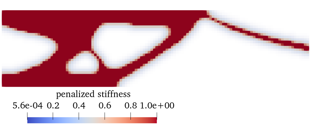
2. Results (density plot)
The users can visualize the optimized densities by opening the <name>.pvd from Paraview.